Using heatmaply to reproduce Nature (2015) Kotsyfakis et al.
Tal Galili
2017-10-17
library(heatmaply)#> Loading required package: plotly#> Loading required package: ggplot2#>
#> Attaching package: 'plotly'#> The following object is masked from 'package:ggplot2':
#>
#> last_plot#> The following object is masked from 'package:stats':
#>
#> filter#> The following object is masked from 'package:graphics':
#>
#> layout#> Loading required package: viridis#> Loading required package: viridisLite#>
#> ---------------------
#> Welcome to heatmaply version 0.11.1
#> Type ?heatmaply for the main documentation.
#> The github page is: https://github.com/talgalili/heatmaply/
#>
#> Suggestions and bug-reports can be submitted at: https://github.com/talgalili/heatmaply/issues
#> Or contact: <tal.galili@gmail.com>
#>
#> To suppress this message use: suppressPackageStartupMessages(library(heatmaply))
#> ---------------------library(dendextend)#>
#> ---------------------
#> Welcome to dendextend version 1.5.2
#> Type citation('dendextend') for how to cite the package.
#>
#> Type browseVignettes(package = 'dendextend') for the package vignette.
#> The github page is: https://github.com/talgalili/dendextend/
#>
#> Suggestions and bug-reports can be submitted at: https://github.com/talgalili/dendextend/issues
#> Or contact: <tal.galili@gmail.com>
#>
#> To suppress this message use: suppressPackageStartupMessages(library(dendextend))
#> ---------------------#>
#> Attaching package: 'dendextend'#> The following object is masked from 'package:stats':
#>
#> cutreeTissue- and time-dependent transcription in Ixodes ricinus salivary glands and midguts when blood feeding on the vertebrate host
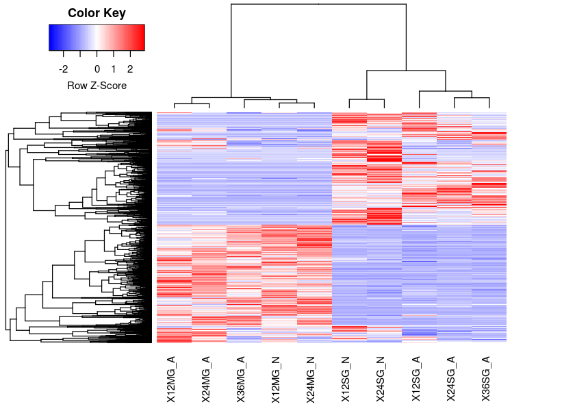
Here we wish to reproduce figure 3: “Figure 3: Heat map of normalized RPKM data from the salivary glands (SG) and midguts (MG) of nymphal and adult Ixodes ricinus fed for different periods of time.”.
The Z score represents the deviation from the mean by standard deviation units. For other details, please see the Figure 2 legend.
Figure 2 legend: A box plot was constructed using normalized reads per kilobase per million (RPKM) values for CDS with a total RPKM (considering the reads of all ten libraries) of 50 or larger to avoid inclusion of poorly expressed contigs. The normalized RPKM values (maximum 100) for ten different libraries from Ixodes ricinus are as follows: the first two numbers indicate the time point of organ collection from 0–12h (12), 12–24h (24), or 24–36h (36). Organs were either salivary glands (SG) or midguts (MG) and developmental stage was either nymphs (N) or adults (A). For more details, please consult the methods.
heatmap.2 of the figure
The data and code for this plot was shared by Ribeiro, Jose (NIH/NIAID) [E]
# rpkm50 <- read.delim("rpkm-50.txt",sep="\t",header=TRUE,dec=".",stringsAsFactors = FALSE,strip.white = TRUE)
### saveRDS(rpkm50, "data\\rpkm50.rda")
# http://r-pkgs.had.co.nz/data.html#data-data
# devtools::use_data(rpkm50)
library(heatmaplyExamples)
data(rpkm50)
head(rpkm50)#> X12SG_N X24SG_N X12SG_A X24SG_A X36SG_A X12MG_N
#> 1 235517.30 201172.23 95552.130 76629.5037 67257.2264 1.575864e+05
#> 2 219038.88 177905.38 81058.734 64990.6312 59070.8028 1.565105e+05
#> 3 207777.50 177673.71 83810.362 67112.6247 58877.7816 1.392322e+05
#> 4 17133.35 37736.14 64136.750 47097.0685 84443.5747 5.659074e+00
#> 5 50284.25 25032.12 1415.041 377.7924 681.7187 5.899005e+00
#> 6 46039.79 43387.75 6213.151 3730.7482 2188.6810 2.961282e+01
#> X24MG_N X12MG_A X24MG_A X36MG_A
#> 1 138293.30600 77681.686190 73534.886550 107423.87800
#> 2 114443.08230 82331.577490 72390.858400 107230.81370
#> 3 121766.27670 68088.353640 64444.787530 94416.34896
#> 4 12.53498 117.556341 16.826781 25.36865
#> 5 0.00000 495.307428 311.971324 0.00000
#> 6 17.16098 1.387416 2.909895 0.00000x <- as.matrix(rpkm50)
rc <- rainbow(nrow(x), start=0, end=.3)
cc <- rainbow(ncol(x), start=0, end=.3)
# pdf(file='heatmap-spearman.pdf')
hr <- hclust(as.dist(1-cor(t(x), method="spearman")), method="complete")# spearman clustering
hc <- hclust(as.dist(1-cor(x, method="spearman")), method="complete")# spearman clustering
library(gplots)#>
#> Attaching package: 'gplots'#> The following object is masked from 'package:stats':
#>
#> lowessheatmap.2(x, col=bluered(75), Colv=as.dendrogram(hc), Rowv=as.dendrogram(hr), scale="row", key=T, keysize=1.5,density.info="none", trace="none",cexCol=0.9, cexRow=0.9,labRow=NA, dendrogram="both") # Z scores
# dev.off()