Using heatmaply with the measles data set
Tal Galili
2017-10-17
library(heatmaply)#> Loading required package: plotly#> Loading required package: ggplot2#>
#> Attaching package: 'plotly'#> The following object is masked from 'package:ggplot2':
#>
#> last_plot#> The following object is masked from 'package:stats':
#>
#> filter#> The following object is masked from 'package:graphics':
#>
#> layout#> Loading required package: viridis#> Loading required package: viridisLite#>
#> ---------------------
#> Welcome to heatmaply version 0.11.1
#> Type ?heatmaply for the main documentation.
#> The github page is: https://github.com/talgalili/heatmaply/
#>
#> Suggestions and bug-reports can be submitted at: https://github.com/talgalili/heatmaply/issues
#> Or contact: <tal.galili@gmail.com>
#>
#> To suppress this message use: suppressPackageStartupMessages(library(heatmaply))
#> ---------------------library(dendextend)#>
#> ---------------------
#> Welcome to dendextend version 1.5.2
#> Type citation('dendextend') for how to cite the package.
#>
#> Type browseVignettes(package = 'dendextend') for the package vignette.
#> The github page is: https://github.com/talgalili/dendextend/
#>
#> Suggestions and bug-reports can be submitted at: https://github.com/talgalili/dendextend/issues
#> Or contact: <tal.galili@gmail.com>
#>
#> To suppress this message use: suppressPackageStartupMessages(library(dendextend))
#> ---------------------#>
#> Attaching package: 'dendextend'#> The following object is masked from 'package:stats':
#>
#> cutreeMeasles
How the data was prepared
Here eval=FALSE as we have the final version in the heatmaplyExamples package.
Preparing the data:
# measles
# bil gates (20 Feb 2015): https://twitter.com/BillGates/status/568749655112228865
# http://graphics.wsj.com/infectious-diseases-and-vaccines/#b02g20t20w15
# http://www.opiniomics.org/recreating-a-famous-visualisation/
# http://www.r-bloggers.com/recreating-the-vaccination-heatmaps-in-r-2/


# source: http://www.r-bloggers.com/recreating-the-vaccination-heatmaps-in-r/
# measles <- read.csv("https://raw.githubusercontent.com/blmoore/blogR/master/data/measles_incidence.csv", header=T,
#                     skip=2, stringsAsFactors=F)
# dir.create("data")
# write.csv(measles, file = "data\\measles.csv")
# measles[measles == "-"] <- NA
measles[,-(1:2)] <- apply(measles[,-(1:2)], 2, as.numeric)

dim(measles)
# head(measles)

d2 <- aggregate(measles, list(measles[, "YEAR"]), "sum", na.rm = T)
rownames(measles) <- d2[,1]
d2 <- d2[, -c(1:4)]
d2 <- t(measles)
# head(measles)

dim(measles)
d2[1:5,1:5]

# head(md2)
#
# # per week
# d22 <- aggregate(measles, list(measles$YEAR, measles$WEEK), "sum", na.rm = T)
# rownames(measles2) <- paste(measles2[,1], d22[,2], sep = "_")
# d22 <- d22[, -c(1:5)]
# d22 <- t(measles2)
# md22 <- reshape2::melt(measles2)
# dim(measles2) # 51 3952
# pander::pander(sqrt(measles))
if(!file.exists("data\\sqrt_d2.csv")) write.csv(sqrt(measles), file = "data\\sqrt_d2.csv")Let’s have measles in a long format.
library(heatmaplyExamples)
data(measles)
dim(measles)
#> [1] 59 72md2 <- reshape2::melt(measles)
head(md2)#> Var1 Var2 value
#> 1 ALABAMA 1930 4389
#> 2 ALASKA 1930 0
#> 3 AMERICAN.SAMOA 1930 0
#> 4 ARIZONA 1930 2107
#> 5 ARKANSAS 1930 996
#> 6 CALIFORNIA 1930 43585Which transformation to use?
We can look at the general timeline trend with different transformations.
library(ggplot2)
ggplot(md2, aes(x = Var2, y = value)) + geom_line(aes(group = Var1)) + geom_smooth(size = 2)
#> `geom_smooth()` using method = 'gam' and formula 'y ~ s(x, bs = "cs")'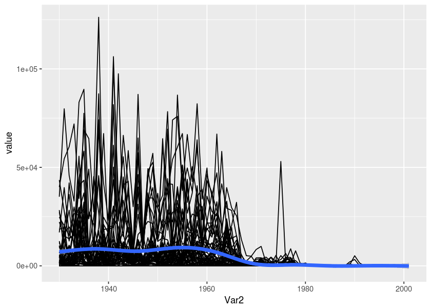
ggplot(md2, aes(x = Var2, y = sqrt(value))) + geom_line(aes(group = Var1)) + geom_smooth(size = 2)#> `geom_smooth()` using method = 'gam' and formula 'y ~ s(x, bs = "cs")'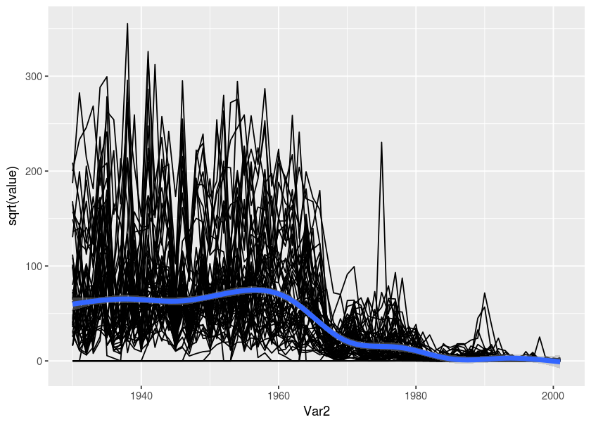
ggplot(md2, aes(x = Var2, y = log(value+.1))) + geom_line(aes(group = Var1)) + geom_smooth(size = 2)#> `geom_smooth()` using method = 'gam' and formula 'y ~ s(x, bs = "cs")'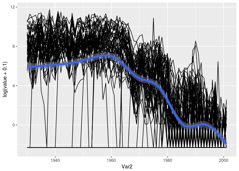
# ggplot(md22, aes(x = Var2, y = value)) + geom_line(aes(group = Var1)) # + geom_smooth(size = 2)

#
# we miss the per state information and the patters of similarity
We can try several heatmaps settings until we get one that works. Notice the effect of the color scheme.
library(gplots)#>
#> Attaching package: 'gplots'#> The following object is masked from 'package:stats':
#>
#> lowesslibrary(viridis)
heatmap.2(measles)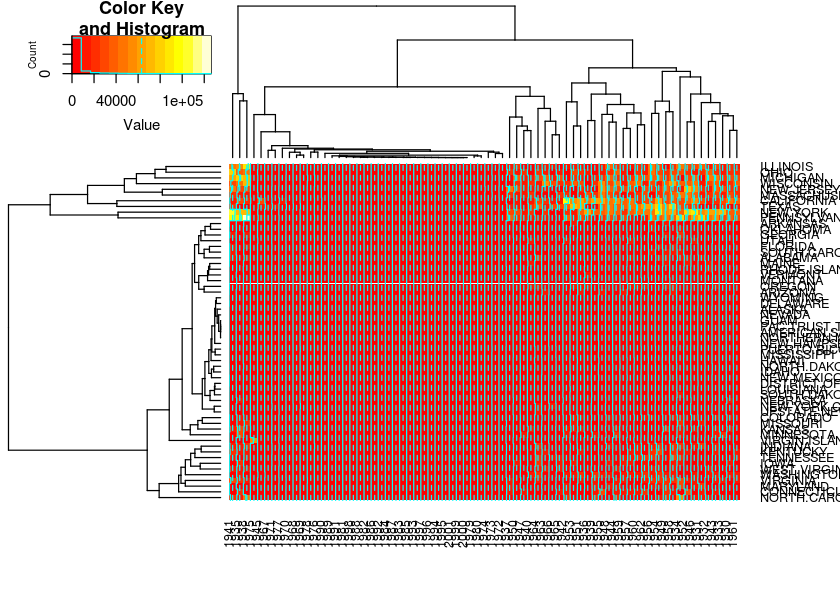
heatmap.2(measles, margins = c(3, 9))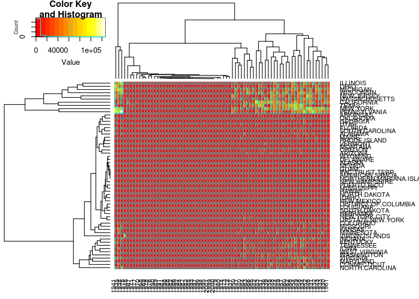
heatmap.2(measles,trace = "none", margins = c(3, 9))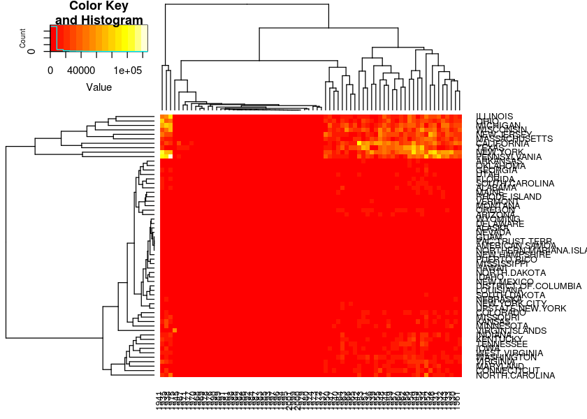
heatmap.2(measles, trace = "none", margins = c(3, 9), dendrogram = "row", Colv = NULL)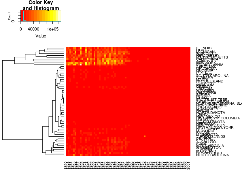
# heatmap.2(sqrt(measles), Colv = NULL, trace = "none", margins = c(3, 9))
library(viridis)
heatmap.2(measles, Colv = NULL, trace = "none", col = viridis(200), margins = c(3, 9))
#> Warning in heatmap.2(measles, Colv = NULL, trace = "none", col =
#> viridis(200), : Discrepancy: Colv is FALSE, while dendrogram is `both'.
#> Omitting column dendogram.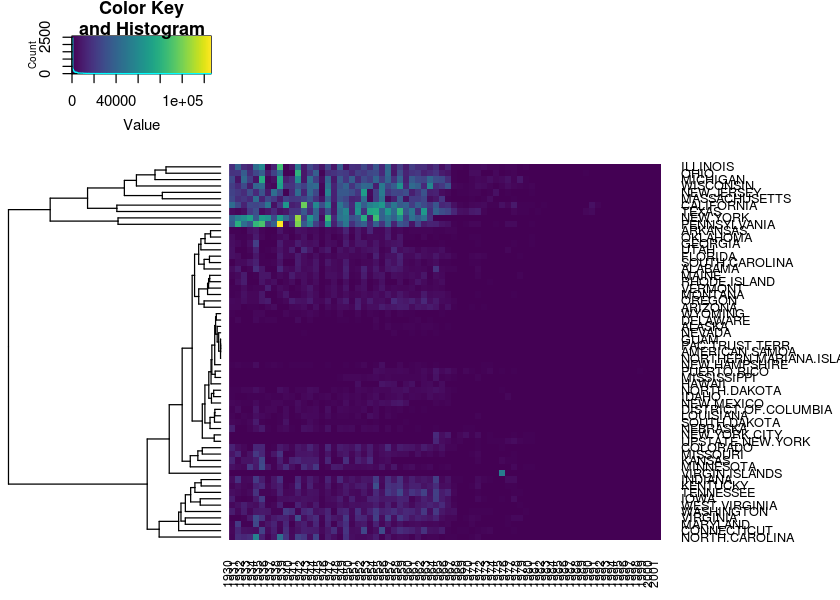
#> Warning in heatmap.2(sqrt(measles), Colv = NULL, trace = "none", col =
#> viridis(200), : Discrepancy: Colv is FALSE, while dendrogram is `both'.
#> Omitting column dendogram.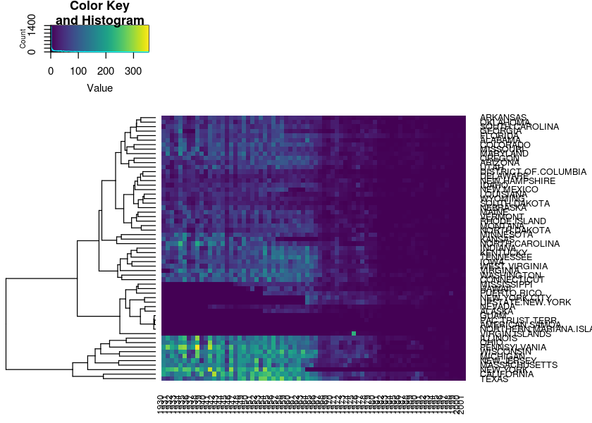
# hist(measles, col = )

library(ggplot2)
library(viridis)
hp <- qplot(x = as.numeric(measles), fill = ..count.., geom = "histogram")
hp + scale_fill_viridis(direction = -1) + xlab("Measles incedence") + theme_bw()
#> `stat_bin()` using `bins = 30`. Pick better value with `binwidth`.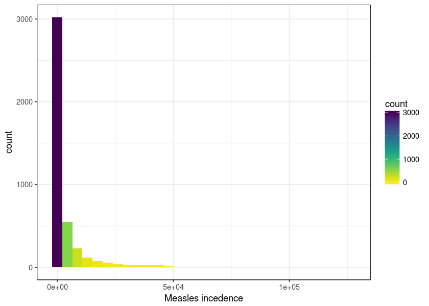
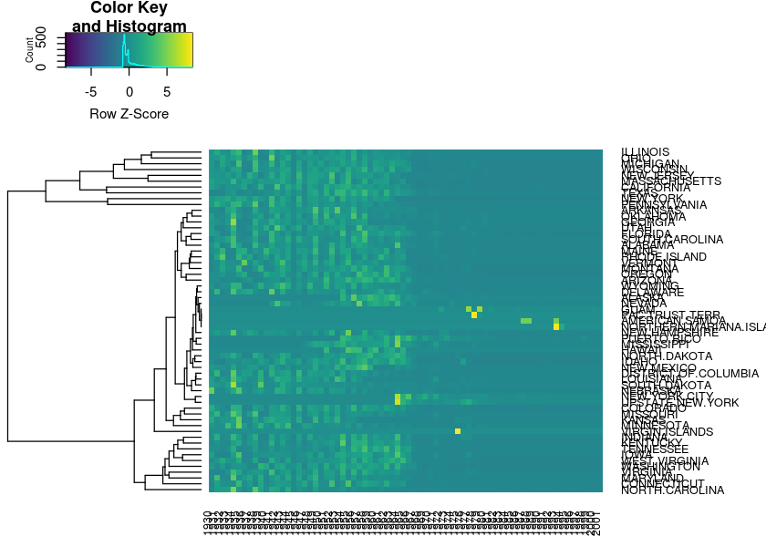
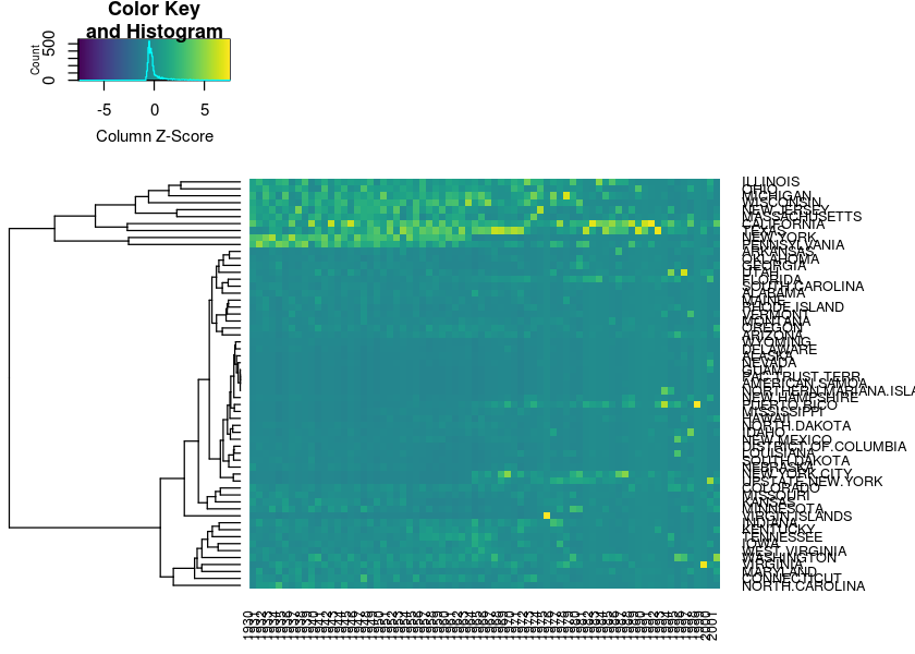
Using scaling doesn’t make much sense in this data.
heatmap.2(measles, dendrogram = "row", Colv = NULL, trace = "none", margins = c(3, 9),
          col = viridis(200),
          scale = "row"
          )
heatmap.2(measles, dendrogram = "row", Colv = NULL, trace = "none", margins = c(3, 9),
          col = viridis(200),
          scale = "column"
          )
Clustering
Decisions for clustering (highlight_branches helps identify the topology of the dendrogram, it colors each branch based on its height):
DATA <- measles
d <- dist(sqrt(DATA))

library(dendextend)
dend_expend(d)[[3]]
#> dist_methods hclust_methods optim
#> 1 unknown ward.D 0.8435986
#> 2 unknown ward.D2 0.8499247
#> 3 unknown single 0.8600853
#> 4 unknown complete 0.8656224
#> 5 unknown average 0.8774877
#> 6 unknown mcquitty 0.8447603
#> 7 unknown median 0.8682800
#> 8 unknown centroid 0.8508883# average seems to make the most sense
dend_row <- d %>% hclust(method = "average") %>% as.dendrogram
dend_row %>% highlight_branches %>% plot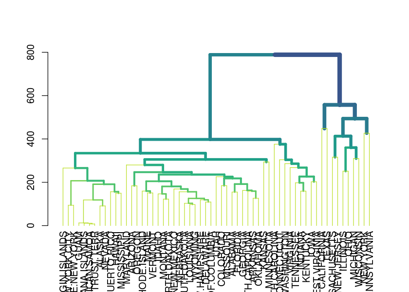
What would be the optimal number of clusters? (it seems that 3 would be good)
library(dendextend)

dend_k <- find_k(dend_row)
plot(dend_k)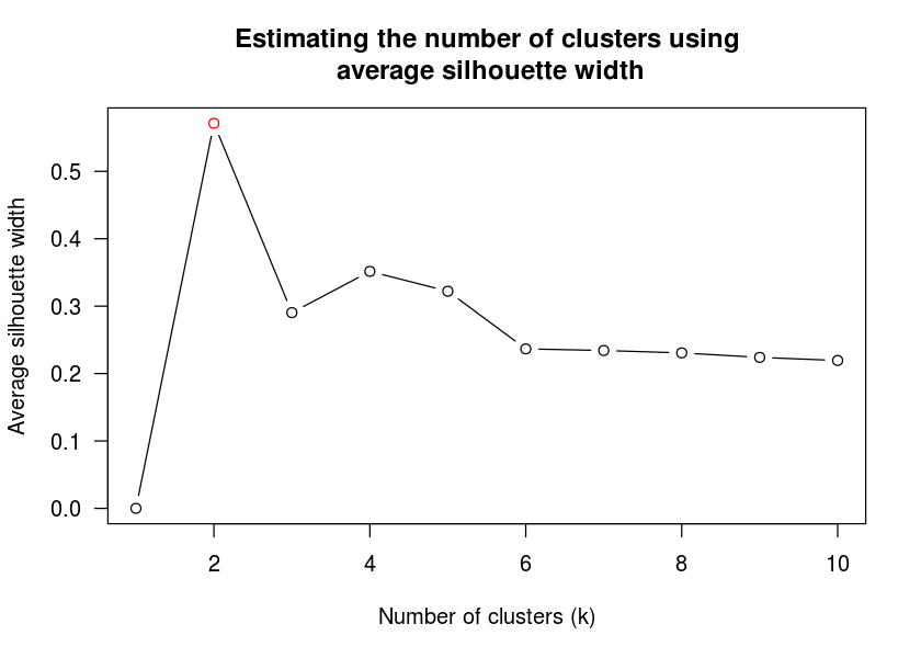
Let’s plot it:
Rowv <- dend_row %>% color_branches(k = 3)
heatmap.2(sqrt(measles), Colv = NULL, Rowv = Rowv, trace = "none", col = viridis(200), margins = c(3, 9))
#> Warning in heatmap.2(sqrt(measles), Colv = NULL, Rowv = Rowv, trace =
#> "none", : Discrepancy: Colv is FALSE, while dendrogram is `both'. Omitting
#> column dendogram.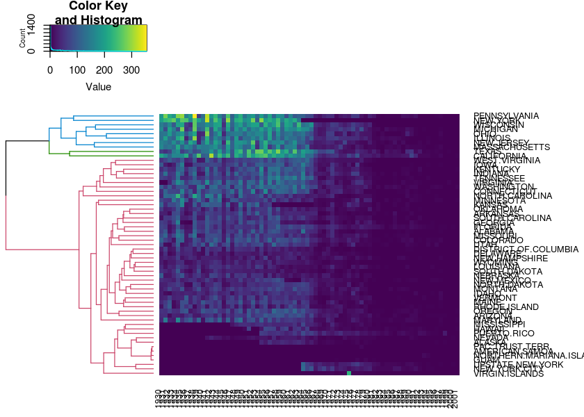
Rowv <- dend_row %>% color_branches(k = 3) %>% seriate_dendrogram(x=d)
heatmap.2(sqrt(measles), Colv = NULL, Rowv = Rowv, trace = "none", col = viridis(200), margins = c(3, 9))
#> Warning in heatmap.2(sqrt(measles), Colv = NULL, Rowv = Rowv, trace =
#> "none", : Discrepancy: Colv is FALSE, while dendrogram is `both'. Omitting
#> column dendogram.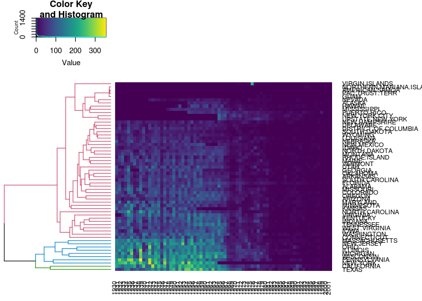
heatmaply
All of this work (other then finding that the hclust method should be average) can simply be done using the following code to produce an interactive heatmap using heatmaply:
library(heatmaply)
heatmaply(sqrt(measles), Colv = NULL, hclust_method = "average",
          fontsize_row = 8,fontsize_col = 6,
          k_row = NA, margins = c(60,170, 70,40),
          xlab = "Year", ylab = "State", main = "Project Tycho's heatmap visualization \nof the measles vaccine"
        )
We can also use plot_method = “plotly”, row_dend_left = TRUE to make the plot more similar to heatmap.2 using the plotly engine (this is a bit more experimental. The default, plot_method = “ggplot”, is often safer to use - but it does not yet support row_dend_left = TRUE properly).
heatmaply(sqrt(measles), Colv = NULL, hclust_method = "average",
          fontsize_row = 8,fontsize_col = 6,
          k_row = NA, margins = c(60,50, 70,90),
          xlab = "Year", ylab = "State", main = "Project Tycho's heatmap visualization \nof the measles vaccine",
          plot_method = "plotly", row_dend_left = TRUE
        )
# save.image("example.Rdata")sessionInfo
sessionInfo()#> R version 3.4.2 (2017-09-28)
#> Platform: x86_64-pc-linux-gnu (64-bit)
#> Running under: Ubuntu 16.04.3 LTS
#>
#> Matrix products: default
#> BLAS: /usr/lib/openblas-base/libblas.so.3
#> LAPACK: /usr/lib/libopenblasp-r0.2.18.so
#>
#> locale:
#> [1] LC_CTYPE=en_GB.UTF-8 LC_NUMERIC=C
#> [3] LC_TIME=en_GB.UTF-8 LC_COLLATE=en_GB.UTF-8
#> [5] LC_MONETARY=en_GB.UTF-8 LC_MESSAGES=en_GB.UTF-8
#> [7] LC_PAPER=en_GB.UTF-8 LC_NAME=C
#> [9] LC_ADDRESS=C LC_TELEPHONE=C
#> [11] LC_MEASUREMENT=en_GB.UTF-8 LC_IDENTIFICATION=C
#>
#> attached base packages:
#> [1] stats graphics grDevices utils datasets methods base
#>
#> other attached packages:
#> [1] gplots_3.0.1 heatmaplyExamples_0.2.0 dendextend_1.5.2
#> [4] heatmaply_0.11.1 viridis_0.4.0 viridisLite_0.2.0
#> [7] plotly_4.7.1 ggplot2_2.2.1.9000
#>
#> loaded via a namespace (and not attached):
#> [1] httr_1.3.1 tidyr_0.6.3 jsonlite_1.5
#> [4] foreach_1.4.3 gtools_3.5.0 shiny_1.0.5
#> [7] assertthat_0.2.0 stats4_3.4.2 yaml_2.1.14
#> [10] robustbase_0.92-7 backports_1.1.0 lattice_0.20-35
#> [13] glue_1.1.1 digest_0.6.12 RColorBrewer_1.1-2
#> [16] colorspace_1.3-2 httpuv_1.3.5 Matrix_1.2-11
#> [19] htmltools_0.3.6 plyr_1.8.4 pkgconfig_2.0.1
#> [22] xtable_1.8-2 purrr_0.2.3 mvtnorm_1.0-6
#> [25] scales_0.5.0.9000 gdata_2.18.0 whisker_0.3-2
#> [28] tibble_1.3.4 mgcv_1.8-22 nnet_7.3-12
#> [31] lazyeval_0.2.0 mime_0.5 magrittr_1.5
#> [34] mclust_5.3 evaluate_0.10.1 nlme_3.1-131
#> [37] MASS_7.3-47 class_7.3-14 tools_3.4.2
#> [40] registry_0.3 data.table_1.10.4 trimcluster_0.1-2
#> [43] stringr_1.2.0 kernlab_0.9-25 munsell_0.4.3
#> [46] cluster_2.0.6 fpc_2.1-10 bindrcpp_0.2
#> [49] compiler_3.4.2 caTools_1.17.1 rlang_0.1.2.9000
#> [52] grid_3.4.2 iterators_1.0.8 htmlwidgets_0.9
#> [55] crosstalk_1.0.0 labeling_0.3 bitops_1.0-6
#> [58] rmarkdown_1.6 gtable_0.2.0 codetools_0.2-15
#> [61] flexmix_2.3-14 TSP_1.1-5 reshape2_1.4.2
#> [64] R6_2.2.2 seriation_1.2-2 gridExtra_2.2.1
#> [67] knitr_1.16 prabclus_2.2-6 dplyr_0.7.2
#> [70] bindr_0.1 rprojroot_1.2 KernSmooth_2.23-15
#> [73] modeltools_0.2-21 stringi_1.1.5 Rcpp_0.12.12
#> [76] gclus_1.3.1 DEoptimR_1.0-8 diptest_0.75-7