Using heatmaply with famous data sets
Tal Galili
2017-10-17
library(heatmaply)#> Loading required package: plotly#> Loading required package: ggplot2#>
#> Attaching package: 'plotly'#> The following object is masked from 'package:ggplot2':
#>
#> last_plot#> The following object is masked from 'package:stats':
#>
#> filter#> The following object is masked from 'package:graphics':
#>
#> layout#> Loading required package: viridis#> Loading required package: viridisLite#>
#> ---------------------
#> Welcome to heatmaply version 0.11.1
#> Type ?heatmaply for the main documentation.
#> The github page is: https://github.com/talgalili/heatmaply/
#>
#> Suggestions and bug-reports can be submitted at: https://github.com/talgalili/heatmaply/issues
#> Or contact: <tal.galili@gmail.com>
#>
#> To suppress this message use: suppressPackageStartupMessages(library(heatmaply))
#> ---------------------library(dendextend)#>
#> ---------------------
#> Welcome to dendextend version 1.5.2
#> Type citation('dendextend') for how to cite the package.
#>
#> Type browseVignettes(package = 'dendextend') for the package vignette.
#> The github page is: https://github.com/talgalili/dendextend/
#>
#> Suggestions and bug-reports can be submitted at: https://github.com/talgalili/dendextend/issues
#> Or contact: <tal.galili@gmail.com>
#>
#> To suppress this message use: suppressPackageStartupMessages(library(dendextend))
#> ---------------------#>
#> Attaching package: 'dendextend'#> The following object is masked from 'package:stats':
#>
#> cutreemtcars - Motor Trend Car Road Tests
The data was extracted from the 1974 Motor Trend US magazine, and comprises fuel consumption and 10 aspects of automobile design and performance for 32 automobiles (1973–74 models).
mtcars2 <- datasets::mtcars
mtcars2$am <- factor(mtcars2$am)
mtcars2$gear <- factor(mtcars2$gear)
mtcars2$vs <- factor(mtcars2$vs)

library(heatmaply)
heatmaply(percentize(mtcars2),
          xlab = "Features", ylab = "Cars",
          main = "Motor Trend Car Road Tests",
          k_col = 2, k_row = NA,
          margins = c(60,100,40,20) )
For visualizing the correlation matrix we wish to use divergent color palette as well as set the limits.
library(heatmaply)

heatmaply(cor(mtcars), margins = c(40, 40, 0, 0),
          k_col = 2, k_row = 2,
          colors = BrBG,
          limits = c(-1,1))
iris - Edgar Anderson’s Iris Data
The famous (Fisher’s or Anderson’s) iris data set gives the measurements in centimeters of the variables sepal length and width and petal length and width, respectively, for 50 flowers from each of 3 species of iris. The species are Iris setosa, versicolor, and virginica. (from
?iris)
The Iris flower data set is fun for learning supervised classification algorithms, and is known as a difficult case for unsupervised learning. Since the values represent length it makes sense to have them start at 0 and end a bit above the highest value in the data-set (which is 7.9).
Notice the use of find_dend and seriate_dendrogram to find the “best” linkage function. Looking at the performance of dend_expend shows that complete gets a cophenetic correlation of 0.72 while the best option (average) gets 0.876.
iris <- datasets::iris

library(heatmaply)
library(dendextend)

iris2 <- iris[,-5]
rownames(iris2) <- 1:150
iris_dist <- iris2 %>% dist
dend <- iris_dist %>% find_dend %>% seriate_dendrogram(., iris_dist)
dend_expend(iris_dist)$performance
#> dist_methods hclust_methods optim
#> 1 unknown ward.D 0.8638236
#> 2 unknown ward.D2 0.8728283
#> 3 unknown single 0.8638787
#> 4 unknown complete 0.7269857
#> 5 unknown average 0.8769561
#> 6 unknown mcquitty 0.8679766
#> 7 unknown median 0.8622006
#> 8 unknown centroid 0.8746715heatmaply(iris, limits = c(0,8),
xlab = "Lengths", ylab = "Flowers",
main = "Edgar Anderson's Iris Data",
Rowv = dend,
margins = c(85, 40),
grid_gap = 0.2, k_row = 3)#> Warning: 'scatter' objects don't have these attributes: 'xgap', 'ygap'
#> Valid attributes include:
#> 'type', 'visible', 'showlegend', 'legendgroup', 'opacity', 'name', 'uid', 'ids', 'customdata', 'hoverinfo', 'hoverlabel', 'stream', 'x', 'x0', 'dx', 'y', 'y0', 'dy', 'text', 'hovertext', 'mode', 'hoveron', 'line', 'connectgaps', 'cliponaxis', 'fill', 'fillcolor', 'marker', 'textposition', 'textfont', 'r', 't', 'error_y', 'error_x', 'xaxis', 'yaxis', 'xcalendar', 'ycalendar', 'idssrc', 'customdatasrc', 'hoverinfosrc', 'xsrc', 'ysrc', 'textsrc', 'hovertextsrc', 'textpositionsrc', 'rsrc', 'tsrc', 'key', 'set', 'frame', 'transforms', '_isNestedKey', '_isSimpleKey', '_isGraticule'New York Air Quality Measurements (airquality)
Daily air quality measurements in New York, May to September 1973.
The plot shows us that most missing values are in the Ozone variable, and the month distribution (available in the row-side notation) shows that most missing values are from June. Notice the use of grid_gap and grey colors in order to aid in the visualization.
library(heatmaply)


airquality2 <- datasets::airquality
airquality2[,c(1:4,6)] <- is.na10(airquality2[,c(1:4,6)])
airquality2[,5] <- factor(airquality2[,5])

heatmaply(airquality2, grid_gap = 1,
            xlab = "Features", ylab = "Days",
            main = "Missing values in 'New York Air Quality Measurements'",
            k_col =3, k_row = 3,
            margins = c(55, 30),
            colors = c("grey80", "grey20"))
#> Warning: 'scatter' objects don't have these attributes: 'xgap', 'ygap'
#> Valid attributes include:
#> 'type', 'visible', 'showlegend', 'legendgroup', 'opacity', 'name', 'uid', 'ids', 'customdata', 'hoverinfo', 'hoverlabel', 'stream', 'x', 'x0', 'dx', 'y', 'y0', 'dy', 'text', 'hovertext', 'mode', 'hoveron', 'line', 'connectgaps', 'cliponaxis', 'fill', 'fillcolor', 'marker', 'textposition', 'textfont', 'r', 't', 'error_y', 'error_x', 'xaxis', 'yaxis', 'xcalendar', 'ycalendar', 'idssrc', 'customdatasrc', 'hoverinfosrc', 'xsrc', 'ysrc', 'textsrc', 'hovertextsrc', 'textpositionsrc', 'rsrc', 'tsrc', 'key', 'set', 'frame', 'transforms', '_isNestedKey', '_isSimpleKey', '_isGraticule'# warning - using grid_color cannot handle a large matrix!
# airquality[1:10,] %>% is.na10 %>%
# heatmaply(color = c("white","black"), grid_color = "grey",
# k_col =3, k_row = 3,
# margins = c(40, 50))
# airquality %>% is.na10 %>%
# heatmaply(color = c("grey80", "grey20"), # grid_color = "grey",
# k_col =3, k_row = 3,
# margins = c(40, 50))
# ALL - Gentleman et al. 2004
Background
This document uses R to analyse an Acute lymphocytic leukemia (ALL) microarray data-set, producing a heatmap (with dendrograms) of genes deferentially expressed between two types of leukemia. The creation of the data and code for static figures is based on the code available from here.
The original citation for the raw data is “Gene expression profile of adult T-cell acute lymphocytic leukemia identifies distinct subsets of patients with different response to therapy and survival” by Chiaretti et al. Blood 2004. (PMID: 14684422). This document demonstrates the recreation of Figure 2 Heatmap from the paper Bioconductor: open software development for computational biology and bioinformatics, Gentleman et al. 2004..
Static cluster heatmap
Getting the data
# Get needed packages:
if(!require("ALL")) {
  source("http://www.bioconductor.org/biocLite.R")
  biocLite("ALL")
}
#> Loading required package: ALL#> Loading required package: Biobase#> Loading required package: BiocGenerics#> Loading required package: parallel#>
#> Attaching package: 'BiocGenerics'#> The following objects are masked from 'package:parallel':
#>
#> clusterApply, clusterApplyLB, clusterCall, clusterEvalQ,
#> clusterExport, clusterMap, parApply, parCapply, parLapply,
#> parLapplyLB, parRapply, parSapply, parSapplyLB#> The following object is masked from 'package:heatmaply':
#>
#> normalize#> The following objects are masked from 'package:stats':
#>
#> IQR, mad, sd, var, xtabs#> The following objects are masked from 'package:base':
#>
#> anyDuplicated, append, as.data.frame, cbind, colMeans,
#> colnames, colSums, do.call, duplicated, eval, evalq, Filter,
#> Find, get, grep, grepl, intersect, is.unsorted, lapply,
#> lengths, Map, mapply, match, mget, order, paste, pmax,
#> pmax.int, pmin, pmin.int, Position, rank, rbind, Reduce,
#> rowMeans, rownames, rowSums, sapply, setdiff, sort, table,
#> tapply, union, unique, unsplit, which, which.max, which.min#> Welcome to Bioconductor
#>
#> Vignettes contain introductory material; view with
#> 'browseVignettes()'. To cite Bioconductor, see
#> 'citation("Biobase")', and for packages 'citation("pkgname")'.if(!require("limma")) {
source("http://www.bioconductor.org/biocLite.R")
biocLite("limma")
}#> Loading required package: limma#>
#> Attaching package: 'limma'#> The following object is masked from 'package:BiocGenerics':
#>
#> plotMAlibrary("ALL")
data("ALL")
eset <- ALL[, ALL$mol.biol %in% c("BCR/ABL", "ALL1/AF4")]
library("limma")
f <- factor(as.character(eset$mol.biol))
design <- model.matrix(~f)
fit <- eBayes(lmFit(eset,design))
selected <- p.adjust(fit$p.value[, 2]) <0.05
esetSel <- eset [selected, ]
color.map <- function(mol.biol) { if (mol.biol=="ALL1/AF4") "#FF0000" else "#0000FF" }
patientcolors <- unlist(lapply(esetSel$mol.bio, color.map))
hm_data <- exprs(esetSel)stats::heatmap
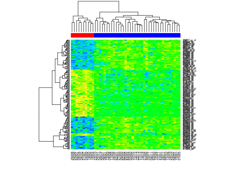
The colors are a bit off compared with the original plot, but they are pretty close.
heatmap(hm_data, col=topo.colors(100), ColSideColors=patientcolors)
gplots::heatmap.2
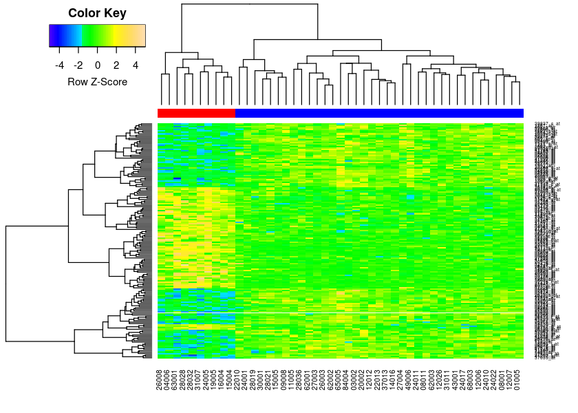
Here also, the colors are a bit off compared with the original plot, but they are pretty close.
library("gplots")#>
#> Attaching package: 'gplots'#> The following object is masked from 'package:stats':
#>
#> lowessheatmap.2(hm_data, col=topo.colors(100), scale="row", ColSideColors=patientcolors,
key=TRUE, symkey=FALSE, density.info="none", trace="none", cexRow=0.5)
Interactive cluster heatmap
heatmaply - replicating gplots::heatmap.2
Several slight changes need to be made. We should use color instead of col, also the seriate parameter should use “mean” and the margin parameter needs to be set. But once done, the results are very similar.
library(heatmaply)


heatmaply(hm_data, color=topo.colors(100), ColSideColors=patientcolors,
          seriate = "mean", scale="row", margin = c(65,120,10,10))
#> Warning in heatmaply.heatmapr(hm, colors = colors, limits = limits,
#> scale_fill_gradient_fun = scale_fill_gradient_fun, : The hover text for
#> col_side_colors is currently not implemented (due to an issue in plotly).
#> We hope this would get resolved in future releases. # %>% layout(autosize = F, width = 500, height = 500)Using heatmaply’s defaults
The heatmaply package tries to offer better defaults.
Instead of topo.colors (or the default “heat.colors” in heatmap.2), heatmaply uses the superior viridis color palette:
library(heatmaply)

heatmaply(hm_data, ColSideColors=patientcolors,
          seriate = "mean", scale="row", margin = c(65,120,10,10))
#> Warning in heatmaply.heatmapr(hm, colors = colors, limits = limits,
#> scale_fill_gradient_fun = scale_fill_gradient_fun, : The hover text for
#> col_side_colors is currently not implemented (due to an issue in plotly).
#> We hope this would get resolved in future releases.Instead of ordering based on the mean, heatmaply uses optimal-leaf-order, and the branches of the dendrograms can be colors to highlight a pre-defined number of assumed clusters:
library(heatmaply)

heatmaply(hm_data, ColSideColors=patientcolors,
          fontsize_row = 5,
          scale="row", margin = c(65,120,10,10),
          k_col = 2, k_row = 5)
#> Warning in heatmaply.heatmapr(hm, colors = colors, limits = limits,
#> scale_fill_gradient_fun = scale_fill_gradient_fun, : The hover text for
#> col_side_colors is currently not implemented (due to an issue in plotly).
#> We hope this would get resolved in future releases.heatmaply(hm_data, ColSideColors=patientcolors,
fontsize_row = 5,
scale="row", margin = c(50,50,10,10),
row_dend_left = TRUE, plot_method = "plotly",
k_col = 2, k_row = 5) votes.repub - Votes for Republican Candidate in Presidential Elections
Background
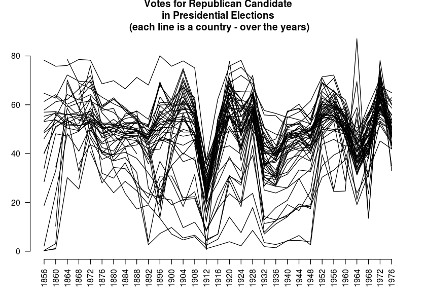
This is a data frame with the percentage of votes given to the republican candidate in presidential elections from 1856 to 1976. Rows represent the 50 states, and columns the 31 elections.
Source: S. Peterson (1973): A Statistical History of the American Presidential Elections. New York: Frederick Ungar Publishing Co. Data from 1964 to 1976 is from R. M. Scammon, American Votes 12, Congressional Quarterly.
Define variables:
votes.repub <- cluster::votes.repubThese data can be visualized using a (costumed made) parallel coordinates plot:
years <- as.numeric(gsub("X", "", colnames(votes.repub)))

par(las = 2, mar = c(4.5, 3, 3, 2) + 0.1, cex = .8)
# MASS::parcoord(votes.repub, var.label = FALSE, lwd = 1)
matplot(1L:ncol(votes.repub), t(votes.repub), type = "l", col = 1, lty = 1,
        axes = F, xlab = "", ylab = "")
axis(1, at = seq_along(years), labels = years)
axis(2)
# Add Title
title("Votes for Republican Candidate\n in Presidential Elections \n (each line is a country - over the years)")
Heatmap
This is a nice example when the parallel coordinates plot has some serious limitations: it does not help us detect the states, we fail to see the missing value patterns, and it is tricky to see clusters in general (due to the large number of threads).
For these data, it can be quite helpful to see a heatmap of the votes across the years. The ordering of the rows is tricky. First, the distance of the vectors (later used for the clustering) should be done after transformation (since we are dealing with proportion of votes). In this case, I used the arcsin transformation (a logit transformation could also work, but the arcsin is safer for dealing with 0/1 observations). But given the clusters, we wish to order the leaves (as much as possible), in order to take into account the missing value clusterings. So we, in fact, have two clusters, one for the raw values, and another for the “shadow matrix” (i.e.: the matrix with 0/1, indicating if a value was missing or not).
# votes.repub[is.na(votes.repub)] <- 50

library(heatmaply)

heatmaply(votes.repub,
          margins = c(60,150,110,10),
          k_row = NA,
          limits = c(0,100),
          main = "Votes for\n Republican Presidential Candidate\n (clustered using complete)",
          srtCol = 60,
          dendrogram = "row",
          ylab = "% Votes for Republican\n Presidential Candidate",
          colors = colorspace::diverge_hcl
         )
# RowSideColors = rev(labels_colors(dend)), # to add nice colored strips animals - Attributes of Animals
Background
This data set considers 6 binary attributes for 20 animals.
see Struyf, Hubert & Rousseeuw (1996), in agnes.
Define variables:
animals <- cluster::animals

colnames(animals) <- c("warm-blooded",
                       "can fly",
                       "vertebrate",
                       "endangered",
                       "live in groups",
                       "have hair")
Heatmap
This is a good example for using a heatmap + colored branches.
# some_col_func <- function(n) rev(colorspace::heat_hcl(n, c = c(80, 30), l = c(30, 90), power = c(1/5, 1.5)))
# some_col_func <- colorspace::diverge_hcl
# some_col_func <- colorspace::sequential_hcl
some_col_func <- function(n) (colorspace::diverge_hcl(n, h = c(246, 40), c = 96, l = c(65, 90)))


library(heatmaply)

heatmaply(as.matrix(animals-1),
          main = "Attributes of Animals",
          srtCol = 35,
          k_col = 3, k_row = 4,
          margins =c(80,50, 40,10),
          col = some_col_func
         )
sessionInfo
sessionInfo()#> R version 3.4.2 (2017-09-28)
#> Platform: x86_64-pc-linux-gnu (64-bit)
#> Running under: Ubuntu 16.04.3 LTS
#>
#> Matrix products: default
#> BLAS: /usr/lib/openblas-base/libblas.so.3
#> LAPACK: /usr/lib/libopenblasp-r0.2.18.so
#>
#> locale:
#> [1] LC_CTYPE=en_GB.UTF-8 LC_NUMERIC=C
#> [3] LC_TIME=en_GB.UTF-8 LC_COLLATE=en_GB.UTF-8
#> [5] LC_MONETARY=en_GB.UTF-8 LC_MESSAGES=en_GB.UTF-8
#> [7] LC_PAPER=en_GB.UTF-8 LC_NAME=C
#> [9] LC_ADDRESS=C LC_TELEPHONE=C
#> [11] LC_MEASUREMENT=en_GB.UTF-8 LC_IDENTIFICATION=C
#>
#> attached base packages:
#> [1] parallel stats graphics grDevices utils datasets methods
#> [8] base
#>
#> other attached packages:
#> [1] gplots_3.0.1 limma_3.32.5 ALL_1.18.0
#> [4] Biobase_2.36.2 BiocGenerics_0.22.0 dendextend_1.5.2
#> [7] heatmaply_0.11.1 viridis_0.4.0 viridisLite_0.2.0
#> [10] plotly_4.7.1 ggplot2_2.2.1.9000
#>
#> loaded via a namespace (and not attached):
#> [1] httr_1.3.1 tidyr_0.6.3 jsonlite_1.5
#> [4] foreach_1.4.3 gtools_3.5.0 shiny_1.0.5
#> [7] assertthat_0.2.0 stats4_3.4.2 yaml_2.1.14
#> [10] robustbase_0.92-7 backports_1.1.0 lattice_0.20-35
#> [13] glue_1.1.1 digest_0.6.12 RColorBrewer_1.1-2
#> [16] colorspace_1.3-2 htmltools_0.3.6 httpuv_1.3.5
#> [19] plyr_1.8.4 pkgconfig_2.0.1 xtable_1.8-2
#> [22] purrr_0.2.3 mvtnorm_1.0-6 scales_0.5.0.9000
#> [25] gdata_2.18.0 whisker_0.3-2 tibble_1.3.4
#> [28] nnet_7.3-12 lazyeval_0.2.0 mime_0.5
#> [31] magrittr_1.5 mclust_5.3 evaluate_0.10.1
#> [34] MASS_7.3-47 class_7.3-14 tools_3.4.2
#> [37] registry_0.3 data.table_1.10.4 trimcluster_0.1-2
#> [40] stringr_1.2.0 kernlab_0.9-25 munsell_0.4.3
#> [43] cluster_2.0.6 fpc_2.1-10 bindrcpp_0.2
#> [46] compiler_3.4.2 caTools_1.17.1 rlang_0.1.2.9000
#> [49] grid_3.4.2 iterators_1.0.8 htmlwidgets_0.9
#> [52] crosstalk_1.0.0 labeling_0.3 bitops_1.0-6
#> [55] rmarkdown_1.6 gtable_0.2.0 codetools_0.2-15
#> [58] flexmix_2.3-14 TSP_1.1-5 reshape2_1.4.2
#> [61] R6_2.2.2 seriation_1.2-2 gridExtra_2.2.1
#> [64] knitr_1.16 prabclus_2.2-6 dplyr_0.7.2
#> [67] bindr_0.1 rprojroot_1.2 KernSmooth_2.23-15
#> [70] modeltools_0.2-21 stringi_1.1.5 Rcpp_0.12.12
#> [73] gclus_1.3.1 DEoptimR_1.0-8 diptest_0.75-7