snifter: fast interpolated t-SNE in R An R package for running openTSNE's implementation of fast interpolated t-SNE.
Source:R/snifter-internal.R, R/snifter.R
snifter.RdSee the openTSNE documentation for further details on these arguments and the general usage of this algorithm.
fitsne(
  x,
  simplified = FALSE,
  n_components = 2L,
  n_jobs = 1L,
  perplexity = 30,
  n_iter = 500L,
  initialization = c("pca", "spectral", "random"),
  neighbors = c("auto", "exact", "annoy", "pynndescent", "approx"),
  negative_gradient_method = c("fft", "bh"),
  learning_rate = "auto",
  early_exaggeration = 250,
  early_exaggeration_iter = 12L,
  exaggeration = NULL,
  dof = 1,
  theta = 0.5,
  n_interpolation_points = 3L,
  min_num_intervals = 50L,
  ints_in_interval = 1,
  metric = "euclidean",
  metric_params = NULL,
  initial_momentum = 0.5,
  final_momentum = 0.8,
  max_grad_norm = NULL,
  random_state = NULL,
  verbose = FALSE
)
Arguments
| x | Input data matrix. |
|---|---|
| simplified | Logical scalar. When |
| n_components | Number of t-SNE components to be produced. |
| n_jobs | Integer scalar specifying the number of corest to be used. |
| perplexity | Numeric scalar controlling the neighborhood used when estimating the embedding. |
| n_iter | Integer scalar specifying the number of iterations to complete. |
| initialization | Character scalar specifying the initialization to use. "pca" may preserve global distance better than other options. |
| neighbors | Character scalar specifying the nearest neighbour algorithm to use. |
| negative_gradient_method | Character scalar specifying the negative gradient approximation to use. "bh", referring to Barnes-Hut, is more appropriate for smaller data sets, while "fft" referring to fast Fourier transform, is more appropriate. |
| learning_rate | Numeric scalar specifying the learning rate, or the
string "auto", which uses |
| early_exaggeration | Numeric scalar specifying the exaggeration factor to use during the early exaggeration phase. Typical values range from 12 to 32. |
| early_exaggeration_iter | Integer scalar specifying the number of iterations to run in the early exaggeration phase. |
| exaggeration | Numeric scalar specifying the exaggeration factor to use during the normal optimization phase. This can be used to form more densely packed clusters and is useful for large data sets. |
| dof | Numeric scalar specifying the degrees of freedom, as described in Kobak et al. “Heavy-tailed kernels reveal a finer cluster structure in t-SNE visualisations”, 2019. |
| theta | Numeric scalar, only used when negative_gradient_method="bh". This is the trade-off parameter between speed and accuracy of the tree approximation method. Typical values range from 0.2 to 0.8. The value 0 indicates that no approximation is to be made and produces exact results also producing longer runtime. |
| n_interpolation_points | Integer scalar, only used when negative_gradient_method="fft". The number of interpolation points to use within each grid cell for interpolation based t-SNE. It is highly recommended leaving this value at the default 3. |
| min_num_intervals | Integer scalar, only used when negative_gradient_method="fft". The minimum number of grid cells to use, regardless of the ints_in_interval parameter. Higher values provide more accurate gradient estimations. |
| ints_in_interval | Numeric scalar, only used when negative_gradient_method="fft". Indicates how large a grid cell should be e.g. a value of 3 indicates a grid side length of 3. Lower values provide more accurate gradient estimations. |
| metric | Character scalar specifying the metric to be used to compute affinities between points in the original space. |
| metric_params | Named list of additional keyword arguments for the metric function. |
| initial_momentum | Numeric scalar specifying the momentum to use during the early exaggeration phase. |
| final_momentum | Numeric scalar specifying the momentum to use during the normal optimization phase. |
| max_grad_norm | Numeric scalar specifying the maximum gradient norm. If the norm exceeds this value, it will be clipped. |
| random_state | Integer scalar specifying the seed used by the random number generator. |
| verbose | Logical scalar controlling verbosity. |
Value
A matrix of t-SNE embeddings.
References
openTSNE: a modular Python library for t-SNE dimensionality reduction and embedding Pavlin G. Poličar, Martin Stražar, Blaž Zupan bioRxiv (2019) 731877; doi: https://doi.org/10.1101/731877
Fast interpolation-based t-SNE for improved visualization of single-cell RNA-seq data George C. Linderman, Manas Rachh, Jeremy G. Hoskins, Stefan Steinerberger, and Yuval Kluger Nature Methods 16, 243–245 (2019) doi: https://doi.org/10.1038/s41592-018-0308-4
Accelerating t-SNE using Tree-Based Algorithms Laurens van der Maaten Journal of Machine Learning Research (2014) http://jmlr.org/papers/v15/vandermaaten14a.html
Examples
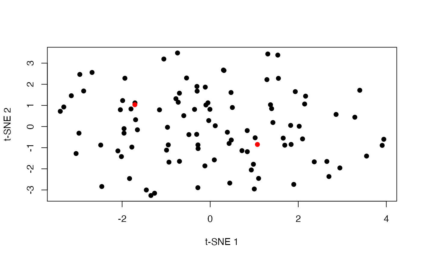
set.seed(42) m <- matrix(rnorm(2000), ncol=20) out <- fitsne(m, random_state = 42L) plot(out, pch = 19, xlab = "t-SNE 1", ylab = "t-SNE 2")## openTSNE allows us to project new points into the existing ## embedding - useful for extremely large data. ## see https://opentsne.readthedocs.io/en/latest/api/index.html out_binding <- fitsne(m[-(1:2), ], random_state = 42L) new_points <- project(out_binding, new = m[1:2, ], old = m[-(1:2), ]) plot(as.matrix(out_binding), col = "black", pch = 19, xlab = "t-SNE 1", ylab = "t-SNE 2")